In a recent post about Mixbus 32c's mixer I discussed some 'issues' with the EQ. I've since discussed this issue with a number of people, including engineers at Harrison.
So the purpose of this post is to clarify some things, correct a potential error, and help you understand (at a very basic level) how and why digital EQs differ.
This doesn't cover EVERYTHING, just one specific difference between EQs in the context of this discussion.
Let's get on with it!
Contents
- What is phase?
- Does phase matter?
- Visualizing Phase
- Harrison Comparison
- Modeling(Simulation) vs Emulation
- Conclusion
- Support Me!
What is phase?
The very first thing you must understand is that all signals can be represented by a sum of sine waves. If you have trouble understanding this, then load up a simple square wave in your DAW and put a spectral analyzer on it. You can easily visualize the harmonic series of sine waves that creates that signal. This is a simplified view of the concept, however it's sufficient to understand the rest of this explanation.
A sine wave can be though of simply as a circle that is unfolded, just like in the animation above. Instead of drawing a circle moving to the right, then to the left... we draw the circle continuing to move to the right. Now we have a sine wave! Just like on a circle, if we trace the sine wave with our finger we can communicate our current position on the circle as a specific 'degree' (or radians). So at the 'top' of the circle or sine, we could say we are at 90°. At the bottom we can say that we're at 270°.
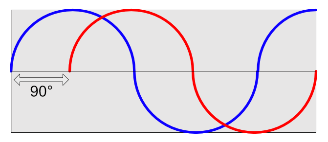
When we only have one signal then we're communicating phase as a position from 0° to some point in the wave. If we have two signals that we're comparing then we're communicating the phase shift. This value is the difference between the position of the 2 sines (of the same frequency). The phase shift amount is communicated in degrees (or radians) relative to the distance traveled to arrive at that phase location in the reference signal. In our image above the red signal is shifted 90° from the blue signal because the red signal starts at 90° on the blue signal.
Not all phase shift is the result of a signal being time shifted, the phase can also be rotated in place.
So if we can view sounds as a summation of sine waves, then we also have to realize that these sine waves may need to start at different times and start at different positions to achieve certain complex sounds. It also means that certain processes can affect the phase of the signals that make up our sound. As these sine waves change phase, they also begin to interact with each other differently, which can have consequences to how we perceive them and their physical characteristics.
Does phase matter?
Go ahead and load up a track in your DAW and flip the polarity on a sound. No difference.
However, when you have relative phase between varying frequencies, things begin to matter. In the Comparator above I have 3 sine waves at 440hz, 460hz and 480hz. The 'NoFlip' file has all 3 playing at a given relative phase. The 'Flip' file has 440hz and 460hz playing at the same relative phase, but 480hz has the polarity inverted (basically similar to a 180° phase rotation).
The difference is subtle, however it is there.
Visual Trickery?
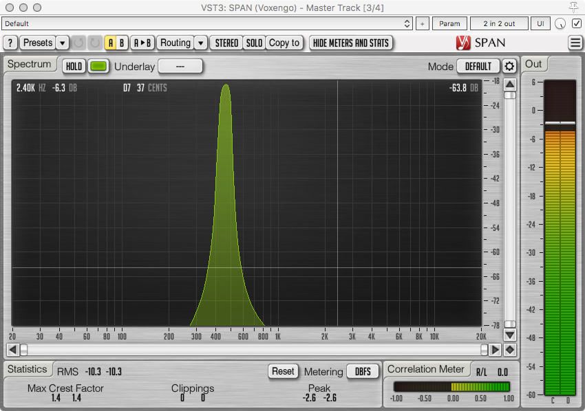
The spectrum shown above is the 440hz, 460hz and 480hz at the same relative phase.
So let's look at it when we flip the polarity (180° phase rotation) of the 480hz signal.
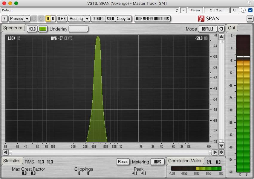
It's the exact same. Despite clearly sounding different, the frequency content is identical. The change in sound is caused by the relative phase change (and some artifacts of our playback system make that more audible).
Peak values
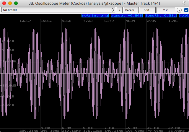
The above is the oscilloscope output of the 440hz, 460hz and 480hz at the same relative phase.
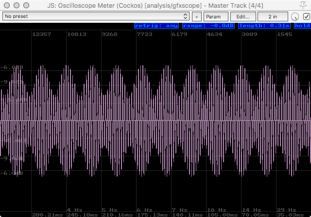
The above is the oscilloscope output of the 440hz, 460hz but the 480hz signal has the polarity reversed.
This may not seem like a big deal (other than that we know they sound slightly different), but now look at the peaks and relative value. Those changes in peak values are going to change how our dynamics processors react to the sound. They also change our overall peak value (though our RMS stays the same!).
Even if the change in sound was not audible, the result of further processing certainly would be audible after processing with processors that are sensitive to amplitude.
Visualizing Phase
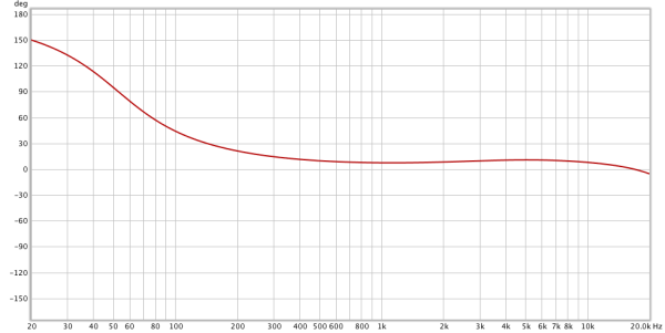
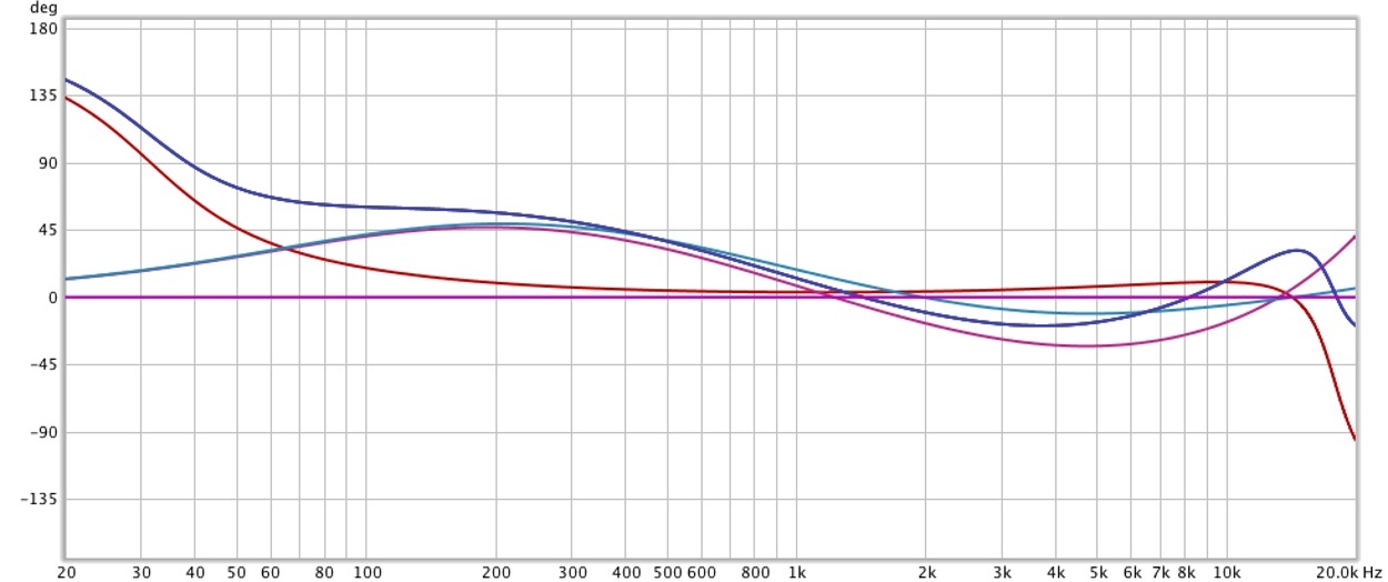
So in order to continue we need to have a way to discuss how to communicate the relative phase changes, at various frequencies, compared to a reference signal. That is where the Bode Phase Plot comes in.
This plot shows the phase change relative to our original signal on the Y axis from -180° to 180°. The X axis shows which frequency has that amount of phase change.
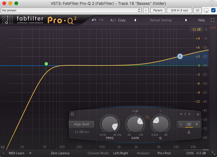
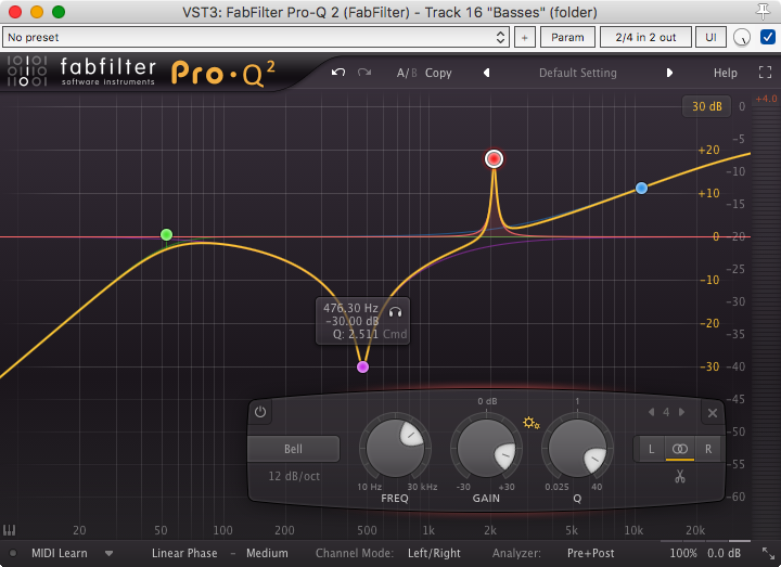
I took an instance of Fabfilter Pro-Q 2 and make a simple highpass and high shelf. Then I measured the phase response of that EQ curve using the Minimal Phase mode, which produces phase shifting at various frequencies (group delay).
In the chart you can see that at 20hz, there is approximately a 150° phase change. At 53hz it's 90°. Around 150hz it's only 30° etc... As we learned above, those phase shifts can be audible if we compared it to another signal with the same frequency response but different phase characteristics... So lets do that!
Here is the Pro-Q 2 EQ curve that produced that phase change. Set in 'Zero Latency' mode (mininum phase)
Deeper in to visualizing phase
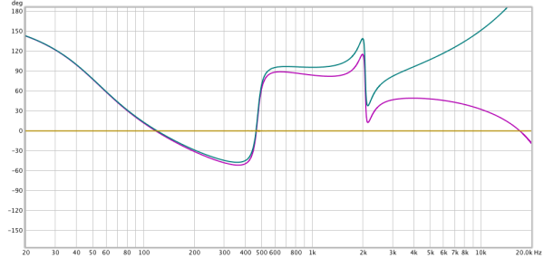
Pro-Q 2 has 3 phase modes. Zero Latency (minimal phase), Natural Phase and Linear Phase. The above phase graph shows the phase response of the same EQ curve.
We can see that obviously the Linear Phase (Yellow) mode has no phase changes. Linear phase has some other tradeoffs though, which we won't discuss here. Fabfilter has a great video on this anyway.
The Zero Latency and Natural Phase modes do differ quite a bit in the high end. This can make quite an audible difference with certain high frequency content like cymbals, certain synth sounds, acoustic stringed instruments or heavily saturated music.
Once again here is the filter that lead to these phase graphs.
Harrison Comparison
Now that you understand that, and how, phase shift (specifically group delay) can make a difference in an EQ, we once again shift back to a complaint I made about Mixbus 32c's channel EQ. Specifically the Filter Cramping at lower sample rates. (All of these tests are at 44.1khz)
This change in the filter shape as you approach the Nyquist Frequency (1/2 the sample rate) obviously can not happen in the analog world because there is no sample rate in the analog world. However when designing digital filters we end up face-butting this frequency wall.
There's a number of potential solutions to this problem if we're trying to create an analog model, however at some point we have to choose between CPU usage, accurate frequency response and accurate phase response. We only get 2 of those, and the third will suffer.
Mixbus vs Pro-Q 2 - Frequency
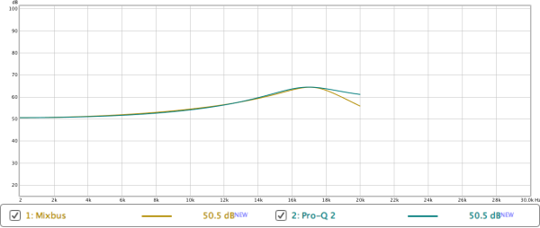
Here's where we get in to the nitty-gritty. I spent a lot of time attempting to match the frequency response of Harrison's 32c High Bell filter with Pro-Q 2. The result is above.
As you can see, it's possible to get very close tho the frequency response of 32c's EQ, except Pro-Q2 does not have that 'cramping' that was discussed. The right side of the filter is not steeper because it is close to the Nyquist Frequency.
But... what does that do to the ever-important phase?
Mixbus vs Pro-Q 2 - Phase
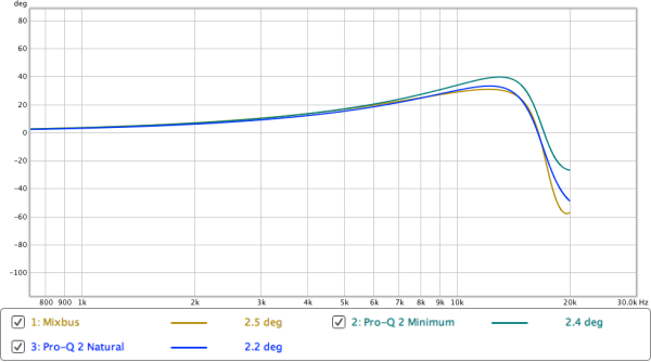
Look at that. Same frequency response (nearly), but our phase response is totally different when comparing Pro-Q 2 Zero latency and Mixbus 32c! The Pro-Q 2 ZL curve has more positive phase shift and less negative. This shows that there is a compensatory filter in Pro-Q 2 that 'fixes' the cramped frequency response, but it also changes our phase response.
Mixbus 32c's phase response on the other hand is very close to what you'd expect to come out of an analog EQ, even if the frequency response is slightly off.
Pro-Q 2's Natural Phase mode is even closer to what you'd expect from an analog EQ, however we have to pay for this small difference with nearly a 3x increase in CPU and a 384 sample (8.7ms @ 44.1khz) latency per instance. That's quite a price to pay for a very small difference, especially when many DAWs do not properly compensate for latency in certain routing setups.
Mixbus 32c's phase response is quite accurate to the analog EQ with very little extra cost.
- NOTE - This also extends to the high and low pass as well, however in that case there is a fairly significant loss of high end that's only avoidable by increasing sample rate.
Modeling(Simulation) vs Emulation
Let's take a short break here to clear something up. There are 2 ways to approach replicating an analog device in the digital world:
- Modeling (Simulation) - Modeling is when you replicate the behaviour of the device without concern for how individual components work, only the result of sections of components, or the whole result.
- Emulation - Emulation is attempting to simulate each component's input and output, then assemble these similar to how the analog device is emulated.
Mixbus 32c, despite some of the marketing claims otherwise, is a Digital Emulation of the 32c channel strip. The designers of Mixbus 32c's channel had the goal of creating the original 32c console's designer's intentions when designing the EQ. Each component in the original was not simulated and combined to create a whole... that is extremely computationally expensive and impractical.
The original designers of the 32c tried their best to avoid saturation, noise, crosstalk and other analog annoyances. The goal of the Mixbus 32c developers was to emulate the design goals of the original 32c channel. To this end it is a success.
However one does have to wonder if some of those unavoidable analog side-effects were part of the charm of the original? I guess you can always add your own noise and saturation if you want ;)
Conclusion
What does this mean? Well, first it means that not all EQs sound the same. They can actually sound quite different sometimes, even with the exact same EQ curves. These differences may be audibly subtle at first, but as we saw there are changes that can greatly affect further processing.
Something that we've also learned is that if our EQ filter is cramped then one of our options is to increase the frequency range afforded to us by our sample rate. Running Mixbus 32c at 48khz or, even better, 96khz allows you to have a de-cramped EQ with a near-perfect analog-like phase response.
While I still have the opinion that the 32c EQ is not particularly useful because the cuts are so wide, it is a good model with some considerations.
- NOTE - I've taken some liberties with terminology and simplification of concepts to the point of being marginally incorrect. This was done in the name of making the subject more easily readable to someone with minimal pre-requisite knowledge. Feel free to point out any errors, but also be aware that some minor things were intentionally twisted slightly to make the concept more easily digestible.
This also isn't EVERYTHING that makes EQ's different. It's just a taste in the context of this post.
Support Me!
This post took 22 hours to research, screenshot, write and edit. If you appreciate the information presented then please consider joining patreon or donating!
If you appreciate the information presented then please consider joining Patreon or donating money/time.